1.2 Physics simulation
Only a brief summary of ArtiSynth physics simulation is described here. Full details are given in [11] and in the related overview paper.
For purposes of physics simulation, the components of a MechModel are grouped as follows:
- Dynamic components
-
Components, such as a particles and rigid bodies, that contain position and velocity state, as well as mass. All dynamic components are instances of the Java interface DynamicComponent. - Force effectors
-
Components, such as springs or finite elements, that exert forces between dynamic components. All force effectors are instances of the Java interface ForceEffector. - Constrainers
-
Components that enforce constraints between dynamic components. All constrainers are instances of the Java interface Constrainer. - Attachments
-
Attachments between dynamic components. While technically these are constraints, they are implemented using a different approach. All attachment components are instances of DynamicAttachment.
The positions, velocities, and forces associated with all the
dynamic components are denoted by the composite vectors
![]() ,
, ![]() , and
, and ![]() .
In addition, the composite mass matrix is given by
.
In addition, the composite mass matrix is given by
![]() .
Newton’s second law then gives
.
Newton’s second law then gives
| (1.1) |
where the ![]() accounts for various “fictitious” forces.
accounts for various “fictitious” forces.
Each integration step involves solving for
the velocities ![]() at time step
at time step ![]() given the velocities and forces
at step
given the velocities and forces
at step ![]() . One way to do this is to solve the expression
. One way to do this is to solve the expression
| (1.2) |
for ![]() , where
, where ![]() is the step size and
is the step size and
![]() . Given the updated velocities
. Given the updated velocities ![]() , one can
determine
, one can
determine ![]() from
from
| (1.3) |
where ![]() accounts for situations (like rigid bodies) where
accounts for situations (like rigid bodies) where ![]() , and then solve for the updated positions using
, and then solve for the updated positions using
| (1.4) |
(1.2) and (1.4) together comprise a simple symplectic Euler integrator.
In addition to forces, bilateral and unilateral constraints give rise to
locally linear constraints on ![]() of the form
of the form
| (1.5) |
Bilateral constraints may include rigid body joints, FEM
incompressibility, and point-surface constraints, while unilateral
constraints include contact and joint limits. Constraints give rise
to constraint forces (in the directions ![]() and
and ![]() )
which supplement the forces of (1.1) in order to enforce
the constraint conditions. In addition, for unilateral constraints,
we have a complementarity condition in which
)
which supplement the forces of (1.1) in order to enforce
the constraint conditions. In addition, for unilateral constraints,
we have a complementarity condition in which ![]() implies no
constraint force, and a constraint force implies
implies no
constraint force, and a constraint force implies ![]() . Any
given constraint usually involves only a few dynamic components and so
. Any
given constraint usually involves only a few dynamic components and so
![]() and
and ![]() are generally sparse.
are generally sparse.
Adding constraints to the velocity solve (1.2) leads to a mixed linear complementarity problem (MLCP) of the form
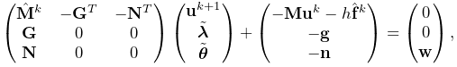 |
|||
| (1.6) |
where ![]() is a slack variable,
is a slack variable, ![]() and
and ![]() give the force
constraint impulses over the time step, and
give the force
constraint impulses over the time step, and ![]() and
and ![]() are
derivative terms defined by
are
derivative terms defined by
| (1.7) |
to account for time variations in ![]() and
and ![]() .
In addition,
.
In addition,
![]() and
and ![]() are
are ![]() and
and ![]() augmented with stiffness
and damping terms terms to accommodate implicit integration, which
is often required for problems involving deformable bodies.
The actual constraint forces
augmented with stiffness
and damping terms terms to accommodate implicit integration, which
is often required for problems involving deformable bodies.
The actual constraint forces ![]() and
and ![]() can be determined
by dividing the impulses by the time step
can be determined
by dividing the impulses by the time step ![]() :
:
| (1.8) |
We note here that ArtiSynth uses a full coordinate formulation, in which the position of each dynamic body is solved using full, or unconstrained, coordinates, with constraint relationships acting to restrict these coordinates. In contrast, some other simulation systems, including OpenSim [7], use reduced coordinates, in which the system dynamics are formulated using a smaller set of coordinates (such as joint angles) that implicitly take the system’s constraints into account. Each methodology has its own advantages. Reduced formulations yield systems with fewer degrees of freedom and no constraint errors. On the other hand, full coordinates make it easier to combine and connect a wide range of components, including rigid bodies and FEM models.
Attachments between components can be implemented by constraining the velocities of the attached components using special constraints of the form
| (1.9) |
where ![]() and
and ![]() denote the velocities of the attached and
non-attached components. The constraint matrix
denote the velocities of the attached and
non-attached components. The constraint matrix ![]() is
sparse, with a non-zero block entry for each master component to
which the attached component is connected. The simplest case involves
attaching a point
is
sparse, with a non-zero block entry for each master component to
which the attached component is connected. The simplest case involves
attaching a point ![]() to another point
to another point ![]() , with the simple velocity relationship
, with the simple velocity relationship
| (1.10) |
That means that ![]() has a single entry of
has a single entry of ![]() (where
(where ![]() is the
is the ![]() identity matrix) in the
identity matrix) in the ![]() -th block column.
Another common case involves connecting a point
-th block column.
Another common case involves connecting a point ![]() to
a rigid frame
to
a rigid frame ![]() . The velocity relationship for this is
. The velocity relationship for this is
| (1.11) |
where ![]() and
and ![]() are the translational and rotational
velocity of the frame and
are the translational and rotational
velocity of the frame and ![]() is the location of the point relative
to the frame’s origin (as seen in world coordinates). The corresponding
is the location of the point relative
to the frame’s origin (as seen in world coordinates). The corresponding
![]() contains a single
contains a single ![]() block entry of the form
block entry of the form
| (1.12) |
in the ![]() block column, where
block column, where
![[l]\equiv\left(\begin{matrix}0&-l_{z}&l_{y}\\
l_{z}&0&-l_{x}\\
-l_{y}&l_{x}&0\end{matrix}\right)](mi/mi1791.png) |
(1.13) |
is a skew-symmetric cross product matrix.
The attachment constraints ![]() could be added directly to
(1.6), but their special form allows us to
explicitly solve for
could be added directly to
(1.6), but their special form allows us to
explicitly solve for ![]() , and hence reduce the size of
(1.6), by factoring out the attached velocities
before solution.
, and hence reduce the size of
(1.6), by factoring out the attached velocities
before solution.
The MLCP (1.6) corresponds to a single step integrator. However, higher order integrators, such as Newmark methods, usually give rise to MLCPs with an equivalent form. Most ArtiSynth integrators use some variation of (1.6) to determine the system velocity at each time step.
To set up (1.6), the MechModel component
hierarchy is traversed and the methods of the different component
types are queried for the required values. Dynamic components (type
DynamicComponent) provide ![]() ,
, ![]() , and
, and ![]() ; force effectors
(ForceEffector) determine
; force effectors
(ForceEffector) determine ![]() and the stiffness/damping
augmentation used to produce
and the stiffness/damping
augmentation used to produce ![]() ; constrainers (Constrainer) supply
; constrainers (Constrainer) supply ![]() ,
, ![]() ,
, ![]() and
and ![]() , and attachments (DynamicAttachment) provide the information needed to factor out
attached velocities.
, and attachments (DynamicAttachment) provide the information needed to factor out
attached velocities.
![[LOGO]](data:image/png;base64,iVBORw0KGgoAAAANSUhEUgAAAAsAAAAOCAYAAAD5YeaVAAAAAXNSR0IArs4c6QAAAAZiS0dEAP8A/wD/oL2nkwAAAAlwSFlzAAALEwAACxMBAJqcGAAAAAd0SU1FB9wKExQZLWTEaOUAAAAddEVYdENvbW1lbnQAQ3JlYXRlZCB3aXRoIFRoZSBHSU1Q72QlbgAAAdpJREFUKM9tkL+L2nAARz9fPZNCKFapUn8kyI0e4iRHSR1Kb8ng0lJw6FYHFwv2LwhOpcWxTjeUunYqOmqd6hEoRDhtDWdA8ApRYsSUCDHNt5ul13vz4w0vWCgUnnEc975arX6ORqN3VqtVZbfbTQC4uEHANM3jSqXymFI6yWazP2KxWAXAL9zCUa1Wy2tXVxheKA9YNoR8Pt+aTqe4FVVVvz05O6MBhqUIBGk8Hn8HAOVy+T+XLJfLS4ZhTiRJgqIoVBRFIoric47jPnmeB1mW/9rr9ZpSSn3Lsmir1fJZlqWlUonKsvwWwD8ymc/nXwVBeLjf7xEKhdBut9Hr9WgmkyGEkJwsy5eHG5vN5g0AKIoCAEgkEkin0wQAfN9/cXPdheu6P33fBwB4ngcAcByHJpPJl+fn54mD3Gg0NrquXxeLRQAAwzAYj8cwTZPwPH9/sVg8PXweDAauqqr2cDjEer1GJBLBZDJBs9mE4zjwfZ85lAGg2+06hmGgXq+j3+/DsixYlgVN03a9Xu8jgCNCyIegIAgx13Vfd7vdu+FweG8YRkjXdWy329+dTgeSJD3ieZ7RNO0VAXAPwDEAO5VKndi2fWrb9jWl9Esul6PZbDY9Go1OZ7PZ9z/lyuD3OozU2wAAAABJRU5ErkJggg==)