10.5 Inverse kinematics
ArtiSynth supplies an inverse kinematic solver, IKSolver, that can be used to compute the configuration of an articulated structure of rigid bodies given the positions of markers attached to those bodies. A primary use of this solver is to transform a marker trajectory, which may not fit the model well due to noise or registration issues, into one that is kinematically feasible given the joint constraints on the bodies. This can be an important preconditioning step for inverse dynamic simulation, as the resulting excitations do not then need to expend effort on infeasible targets.
10.5.1 Inverse kinematics solver
An IKSolver is created with the following constructors:
| IKSolver (MechModel mech, Collection<? extends Marker> mkrs) | |
| IKSolver (MechModel mech, Collection<? extends Marker> mkrs, VectorNd weights) |
mech is the MechModel containing the bodies and constraints, mkrs is a list of markers, and weights is an optional set of marker weight values. If weights is not specified, markers are assumed to have a weight of 1. Each marker is assumed to be either a FrameMarker or GenericMarker that is attached to a RigidBody; other marker types will cause an exception to be thrown. The solver finds all the rigid bodies attached to the specified markers, together with all body connectors (Section 3.4.3) constraining the motion of those bodies, plus any additional bodies connected to the arrangement via connectors.
The solver does not account for the following:
- 1.
Non-rigid bodies, such as FEM models, that might be attached to some of the connectors;
- 2.
Contact constraints.
After the solver is created, the resulting component configuration can be queried with the following methods:
| MechModel getMechModel() |
Returns the MechModel. |
| int numMarkers() |
Returns the number of markers. |
| ArrayList<Marker> getMarkers() |
Returns the markers. |
| VectorNd getMarkerWeights() |
Returns the marker weights. |
| void setMarkerWeights(VectorNd wgts) |
Sets the marker weights. |
| int numBodies() |
Returns the number of connected bodies. |
| ArrayList<RigidBody> getBodies() |
Returns the connected bodies. |
| ArrayList<RigidTransform3d> getBodyPoses() |
Returns the poses of the connected bodies. |
| ArrayList<RigidBody> getBodies() |
Returns the bodies attached to markers. |
| ArrayList<BodyConstrainer> getConstrainers() |
Returns all constrainers and connectors linking the bodies. |
The application can then use the method
| int solve (VectorNd mtargs) |
to set the body poses (and hence marker positions) so as to minimize the error
between the marker target positions specified by mtargs and the feasible
marker positions. mtargs supplies the target positions as a composite
vector of size ![]() , where
, where ![]() is the value returned by numMarkers(), and the method returns either the number of iterations required
for the solve, or -1 if the solve did not convergence to the required
tolerance.
is the value returned by numMarkers(), and the method returns either the number of iterations required
for the solve, or -1 if the solve did not convergence to the required
tolerance.
When using the IKSolver, it is sometimes necessary to explicitly identify some bodies as being “grounded”, in the sense that they should not be moved by the solver. This can be done by setting the grounded property of the body to true. (In a dynamic simulation, grounded bodies are often those whose dynamic property is false. However, this property is not meaningful in the context of an IK solve, and so the grounded property substitutes for this.)
Since solve() modifies the positions of the bodies associated with the solver, it changes the state of the MechModel. In order to leave the MechModel state unchanged, an application can call the solver methods saveModelState() and restoreModelState() before and after the use of solve().
An as example, the following code processes a trajectory of marker positions by calling solve() in a loop:
IKSolver exports a number of methods related to the solution process:
| double getConvergenceTol() |
Returns the convergence tolerance. |
| void setConvergenceTol (double tol) |
Sets the convergence tolerance. |
| int getMaxIterations() |
Returns the maximum number of solve iterations. |
| void setMaxIterations (int maxi) |
Sets the maximum number of solve iterations. |
| void saveModelState() |
Saves the MechModel state internally. |
| void restoreModelState() |
Restores MechModel state to that saved internally. |
The default values for the convergence tolerance and maximum number of
iterations are ![]() and 30.
and 30.
10.5.2 Creating probes with IKSolver
IKSolver supplies the following methods that use its solve() method to convert probes of target marker positions into PositionInputProbes of feasible markers positions or body poses:
In these methods, name is an optional probe name, targProbe is a probe containing the target positions for the markers, targDataFilePath is a path to a probe file (Section 5.4.4) containing target position data, useTargetProps specifies whether the probe should be bound to target properties (Section 5.4.8), rotRep is an instance of RotationRep, which indicates how rotations should be represented (Section 5.4.8), and interval is the time spacing between knots in the created probe. The created probe’s start and stop time is taken from the input probe.
These probe creation methods take care to save and restore the MechModel state.
The only restriction on the targProbe used by these methods is that its data vector size is
, where
is the number of markers associated with the solver.
These methods transform target marker data into position probes for either markers or body poses that are kinematically feasible. In the following example, a TRCReader (Section 5.5.1) is used to create a marker probe from a TRC file and transform it into a feasible marker position probe:
10.5.3 Using IKSolver in a simulation context
Much of the discussion above entails using IKSolver in a stand-alone manner (perhaps in a model’s build() method) that is independent of an actual simulation. However, there may be situations in which one wishes to use the solver to update body and marker positions as a simulation progresses.
One way to do this would be to define a Controller (Section 5.3) that calls the solve() method inside its apply() method. Marker targets would have to be supplied to solver in some way, and it would necessary to ensure that the bodies being controlled by the solver have their dynamic property set to false. IKSolver supplies some convenience methods to manage this:
| void setBodiesDynamic (boolean dynamic) |
Sets dynamic property for all bodies. |
| void resetBodiesDynamic() |
Resets dynamic property for bodies to their initial state. |
Another way to use IKSolver in a simulation is to use an IKProbe, which embeds an IKSolver inside aNumericControlProbe. An IKProbe can be created with the following constructors:
where name is an optional probe name, fileName is a probe file containing probe data, startTime and stopTime set the probe’s start and stop times, and the other arguments mirror those of the IKSolver constructors (wgts can be null if not needed).
If the second constructor is used, the probe is created with only two data points at its start and end (reflecting the current marker positions), and so the actual trajectory data must be added. One way to do this would be to use one of the probe’s addData() methods:
The method setBodiesDynamic() is one of several IKSolver methods that are passed on by IKProbe, including resetBodiesDynamic(), set/getConvergenceTol(), set/getMaxIterations(), numMarkers(), and getMarkers(). IKProbe also maintains the property bodiesNonDynamicIfActive, which ensures that the probe automatically calls setBodiesDynamic(false) when it becomes active and resetBodiesDynamic() when it becomes inactive.
Another way to set IKProbe data is to simply copy it from another probe using setValues(), as described in Section 5.4.5. For example:
10.5.4 Example: moving MultiJointedArm with an IKProbe
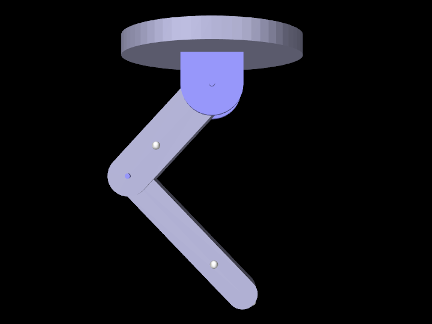
The example model artisynth.demos.tutorial.IKMultiJointedArm shows how to move the MultiJointedArm model (Section 3.5.16) using an IKProbe and marker target data read from a TRC file. This is essentially the same demo as TRCMultiJointedArm (Section 5.5.3), except that it uses inverse kinematics instead of a crude physical simulation in which the markers are connected to the target points by springs. The source code for the build() method is shown below:
Since the model extends MultiJointedArm, build() first calls super.build() to create that model. Next, as in TRCMultiJointedArm, a TRC file containing the marker trajectories is read (lines 5-7). Next, an IKProbe is created to control the markers, with its start and stop times determined directly from the TRC frame times (lines 10-16).
To illustrate a different way of setting probe data, the marker positions for each frame are extracted directly from the TRC reader and added to the probe using addData(t,vec) (lines 19-24). The probe’s bodiesNonDynamicIfActive property is also set (line 27) to ensure that the rigid bodies are set non-dynamic when the probe is active.
To run this example in ArtiSynth, select All demos > tutorial > IKMultiJointedArm from the Models menu.
10.5.5 Example: controlling ToyMuscleArm with inverse kinematics
The final example in this chapter also involves using the tracking controller to move ToyMuscleArm. Several marker targets are used, driven by data read from a TRC file, an IKSolver transforms the data into a feasible trajectory, and the data is used to create velocity targets that when combined with PD control reduce the tracking error. The model is
artisynth.demos.tutorial.IKInverseMuscleArm
and its class definition, excluding import statements, is shown below:
The build() method starts by setting up a tracking controller in the same manner as for InverseMuscleArm (Section 10.2.4) (lines 10-18). Next, the base body is marked as “ground” by setting its grounded property (line 20); this is necessary to prevent the IKSolver from moving it.
This example tracks three markers with component numbers 8, 0, and 2. These are collected into the list markers and added to the controller as targets (lines 20-36). A target position probe containing the marker trajectory, and attached to the tracking controller target points, is then created directly from the TRC file (lines 41-46). Since this file contains data for all the markers, we specify the markers we want using the label list mkrLabels which was created from their numbers.
To filter the marker data (which for this example has been deliberately misregistered), an IKSolver is created and used to create an input probe containing a feasible trajectory (lines 49-51). The data from this probe is then used to overwrite that of the target position probe (line 53). After this is done, the target position probe is differentiated to create a target velocity probe (lines 56-59). To take advantage of this velocity information, the controller is configured to use PD control (lines 62-65) with constants that were tuned manually. Lastly, an output probe is created to record the excitations, and another is created to observe both the target and actual position of the distal marker (which appears first in markers).
To run this example in ArtiSynth, select All demos > tutorial > IKInverseMuscleArm from the Models menu. A view of the timeline, showing the four probes, is given in Figure 10.19. Figure 10.20 (left) shows the resulting excitations, while Figure 10.20 (right) shows the different excitations produced if the target trajectory is left unfiltered. (To run with an unfiltered trajectory, comment out line 53. The model with then appear as in Figure 10.18, right). Finally, Figure 10.21 shows two outputs of the “distal tracking” probe, the left one with velocity information available to the controller, and the right one with it removed (which can be done interactively by making the target velocity probe inactive). Without velocity information, the marker lags the target by a noticeable amount.
![[LOGO]](data:image/png;base64,iVBORw0KGgoAAAANSUhEUgAAAAsAAAAOCAYAAAD5YeaVAAAAAXNSR0IArs4c6QAAAAZiS0dEAP8A/wD/oL2nkwAAAAlwSFlzAAALEwAACxMBAJqcGAAAAAd0SU1FB9wKExQZLWTEaOUAAAAddEVYdENvbW1lbnQAQ3JlYXRlZCB3aXRoIFRoZSBHSU1Q72QlbgAAAdpJREFUKM9tkL+L2nAARz9fPZNCKFapUn8kyI0e4iRHSR1Kb8ng0lJw6FYHFwv2LwhOpcWxTjeUunYqOmqd6hEoRDhtDWdA8ApRYsSUCDHNt5ul13vz4w0vWCgUnnEc975arX6ORqN3VqtVZbfbTQC4uEHANM3jSqXymFI6yWazP2KxWAXAL9zCUa1Wy2tXVxheKA9YNoR8Pt+aTqe4FVVVvz05O6MBhqUIBGk8Hn8HAOVy+T+XLJfLS4ZhTiRJgqIoVBRFIoric47jPnmeB1mW/9rr9ZpSSn3Lsmir1fJZlqWlUonKsvwWwD8ymc/nXwVBeLjf7xEKhdBut9Hr9WgmkyGEkJwsy5eHG5vN5g0AKIoCAEgkEkin0wQAfN9/cXPdheu6P33fBwB4ngcAcByHJpPJl+fn54mD3Gg0NrquXxeLRQAAwzAYj8cwTZPwPH9/sVg8PXweDAauqqr2cDjEer1GJBLBZDJBs9mE4zjwfZ85lAGg2+06hmGgXq+j3+/DsixYlgVN03a9Xu8jgCNCyIegIAgx13Vfd7vdu+FweG8YRkjXdWy329+dTgeSJD3ieZ7RNO0VAXAPwDEAO5VKndi2fWrb9jWl9Esul6PZbDY9Go1OZ7PZ9z/lyuD3OozU2wAAAABJRU5ErkJggg==)